CytoSig#

To facilitate the interpretation of scRNA-seq gene expression readouts and their differences across conditions we can summarize the information and infer pathway activities from prior knowledge.

In this notebook we use decoupler [Badia-I-Mompel et al., 2022], a tool that contains different statistical methods to extract biological activities from omics data using prior knowledge. We run the method on the results from the differential gene expression analysis that compared scRNAseq data from LUAD and LUSC using celltype specific pseudo-bulk data.

Note

Curated gene sets are readily available from MSigDB [Liberzon et al., 2015] and include amongst others gene ontology (GO)-terms [Consortium, 2004], KEGG [Kanehisa, 2000] pathways and Reactome [Gillespie et al., 2021] pathways. In addition, several recent efforts focus on the curation of high-quality gene signatures: PROGENy [Schubert et al., 2018] provides a set of reliable signatures for 14 cancer pathways derived from hundreds of perturbation experiments. Unlike signatures based on genes directly involved in a pathway (e.g. from KEGG), these signatures consist of downstream “pathway-responsive genes” that are differentially expressed when the pathway is perturbed (figure 1.10). This is beneficial as pathways tend to be regulated via post-translational modifications. Naturally, these modifications cannot be measured using RNA-sequencing, but requires either phosphoproteomics or targeted antibody assays. CytoSig [Jiang et al., 2021] is a similar effort focussing on cytokine signaling signatures. Based on more than 2000 cytokine treatment experiments, the authors derived 52 signatures. DoRothEA [Garcia-Alonso et al., 2019] integrates transcription factor activity signatures from manually curated resources, large-scale experiments

We infer activities of the following types:

Pathways from PROGENy [Schubert et al., 2018]
Transcription factors from DoRothEA [Garcia-Alonso et al., 2019]
Molecular Signatures (MSigDB) [Liberzon et al., 2015]
Cytokine signaling (CytoSig) [Jiang et al., 2021]

%load_ext autoreload
%autoreload 2

import os
import re
import urllib.request
from pathlib import Path

import decoupler as dc
import matplotlib.pyplot as plt
import numpy as np
import pandas as pd
import scanpy as sc
import seaborn as sns
import statsmodels.stats.multitest
from IPython.display import display

import atlas_protocol_scripts as aps

1. Configure paths#

Define paths to input files
- adata_path: Path to anndata file
- deseq_path: Path to directory where DESeq2 differential expression results are stored

adata_path = "../../data/input_data_zenodo/atlas-integrated-annotated.h5ad"
deseq_path = "../../data/results/differential_expression"

Define and create output directory

results_dir = "../../data/results/10_functional_analysis"
os.makedirs(results_dir, mode=0o750, exist_ok=True)

Define paths to network/model files. These will be automatically downloaded and stored in these files in a later step.

tfnet_file = Path(results_dir, "tf_net_dorothea_hs.tsv")
pwnet_file = Path(results_dir, "pw_net_progeny_hs.tsv")
msigdb_file = Path(results_dir, "msigdb_hs.tsv")
cytosig_file = Path(results_dir, "cytosig_signature.tsv")

2. Load data#

Load AnnData object

adata = sc.read_h5ad(adata_path)

print(f"Anndata has: {adata.shape[0]} cells and {adata.shape[1]} genes")

Anndata has: 62119 cells and 17837 genes

Retrieve and load DoRothEA data. We limit the analysis to the three highest confidence levels A, B and C.

if tfnet_file.exists():
    tfnet = pd.read_csv(tfnet_file, sep="\t")
else:
    tfnet = dc.get_dorothea(organism="human", levels=["A", "B", "C"])
    tfnet.to_csv(tfnet_file, sep="\t", index=False)

Retrieve and load PROGENy data

# Retrieve Progeny db
if pwnet_file.exists():
    pwnet = pd.read_csv(pwnet_file, sep="\t")
else:
    pwnet = dc.get_progeny(organism="human", top=100)
    pwnet.to_csv(pwnet_file, sep="\t", index=False)

Retrieve and load data from MSigDB. Here, we filter for the “hallmark” gene sets.

# Retrieve MSigDB resource
if msigdb_file.exists():
    msigdb = pd.read_csv(msigdb_file, sep="\t")
else:
    msigdb = dc.get_resource("MSigDB")

    # Filter by a desired geneset collection, for example hallmarks
    msigdb = msigdb[msigdb["collection"] == "hallmark"]
    msigdb = msigdb.drop_duplicates(["geneset", "genesymbol"])

    msigdb.to_csv(msigdb_file, sep="\t", index=False)

Retrieve and load the CytoSig signatures

# Retrieve CytoSig signature
if cytosig_file.exists():
    cytosig_signature = pd.read_csv(cytosig_file, sep="\t")
else:
    urllib.request.urlretrieve(
        "https://github.com/data2intelligence/CytoSig/raw/master/CytoSig/signature.centroid.expand",
        cytosig_file,
    )
    cytosig_signature = pd.read_csv(cytosig_file, sep="\t")

3. Define contrasts#

Here we define the gene expression contrasts/comparisons for which we to run the functional analyses.

contrasts is a list of dicts with the following keys:

name: contrast name
condition: test group
reference: reference group

For this tutorial, we only show one single comparison: LUAD vs. LUSC.

contrasts = [
    {"name": "LUAD_vs_LUSC", "condition": "LUAD", "reference": "LUSC"},
]
contrasts

[{'name': 'LUAD_vs_LUSC', 'condition': 'LUAD', 'reference': 'LUSC'}]

Create result directories for each contrast

for contrast in contrasts:
    res_dir = Path(results_dir, contrast["name"].replace(" ", "_"))
    os.makedirs(res_dir, mode=0o750, exist_ok=True)
    contrast["res_dir"] = res_dir

Define column in adata.obs that contains the desired cell-type annotation. This must match the column used in the Differential gene expression section.

cell_type_class = "cell_type_coarse"

Make list of all cell types in the specified column

cell_types = adata.obs[cell_type_class].unique()
print(f"Cell types in {cell_type_class} annotation:\n")
for ct in cell_types:
    print(ct)

Cell types in cell_type_coarse annotation:

B cell
T cell
Epithelial cell
Macrophage/Monocyte
Mast cell
Plasma cell
cDC
Stromal
NK cell
Endothelial cell
pDC
Neutrophils

4. Read DESeq2 results#

Load TSV files created in the Differential gene expression step.

for contrast in contrasts:
    print(f"Working on: {contrast['name']}")

    de_res = {}

    for ct in cell_types:
        ct_fs = re.sub("[^0-9a-zA-Z]+", "_", ct)
        deseq_file = Path(deseq_path, contrast["name"], ct_fs, ct_fs + "_DESeq2_result.tsv")
        if os.path.exists(deseq_file):
            print(f"Reading DESeq2 result for {ct}: {deseq_file}")
            de_res[ct] = pd.read_csv(deseq_file, sep="\t").assign(cell_type=ct)
        else:
            print(f"No DESeq2 result found for: {ct}")

    contrast["cell_types"] = de_res.keys()
    contrast["de_res"] = de_res

Working on: LUAD_vs_LUSC
Reading DESeq2 result for B cell: ../../data/results/differential_expression/LUAD_vs_LUSC/B_cell/B_cell_DESeq2_result.tsv
Reading DESeq2 result for T cell: ../../data/results/differential_expression/LUAD_vs_LUSC/T_cell/T_cell_DESeq2_result.tsv
Reading DESeq2 result for Epithelial cell: ../../data/results/differential_expression/LUAD_vs_LUSC/Epithelial_cell/Epithelial_cell_DESeq2_result.tsv
Reading DESeq2 result for Macrophage/Monocyte: ../../data/results/differential_expression/LUAD_vs_LUSC/Macrophage_Monocyte/Macrophage_Monocyte_DESeq2_result.tsv
Reading DESeq2 result for Mast cell: ../../data/results/differential_expression/LUAD_vs_LUSC/Mast_cell/Mast_cell_DESeq2_result.tsv
Reading DESeq2 result for Plasma cell: ../../data/results/differential_expression/LUAD_vs_LUSC/Plasma_cell/Plasma_cell_DESeq2_result.tsv
Reading DESeq2 result for cDC: ../../data/results/differential_expression/LUAD_vs_LUSC/cDC/cDC_DESeq2_result.tsv
Reading DESeq2 result for Stromal: ../../data/results/differential_expression/LUAD_vs_LUSC/Stromal/Stromal_DESeq2_result.tsv
Reading DESeq2 result for NK cell: ../../data/results/differential_expression/LUAD_vs_LUSC/NK_cell/NK_cell_DESeq2_result.tsv
Reading DESeq2 result for Endothelial cell: ../../data/results/differential_expression/LUAD_vs_LUSC/Endothelial_cell/Endothelial_cell_DESeq2_result.tsv
No DESeq2 result found for: pDC
Reading DESeq2 result for Neutrophils: ../../data/results/differential_expression/LUAD_vs_LUSC/Neutrophils/Neutrophils_DESeq2_result.tsv

Convert DE results to p-value/logFC/stat matrices as used by decoupler

# Concat and build the stat matrix
for contrast in contrasts:
    lfc_mat, fdr_mat = aps.tl.long_form_df_to_decoupler(pd.concat(contrast["de_res"].values()), p_col="padj")
    stat_mat, _ = aps.tl.long_form_df_to_decoupler(
        pd.concat(contrast["de_res"].values()), log_fc_col="stat", p_col="padj"
    )
    contrast["lfc_mat"] = lfc_mat
    contrast["stat_mat"] = stat_mat
    contrast["fdr_mat"] = fdr_mat
    display(lfc_mat)
    display(fdr_mat)
    display(stat_mat)

gene_id	A1BG	A1BG-AS1	A2M	A2M-AS1	A2ML1	A4GALT	A4GNT	AAAS	AACS	AADAC	...	ZW10	ZWILCH	ZWINT	ZXDA	ZXDB	ZXDC	ZYG11A	ZYG11B	ZYX	ZZEF1
cell_type
B cell	-0.363007	-0.906790	-0.934158	0.000000	0.000000	1.306582	0.000000	0.783459	0.511908	0.000000	...	1.573657	-0.915355	3.137976	-0.539899	-0.685941	-0.482270	-1.651918	1.164252	-0.682958	-0.776318
Endothelial cell	0.833616	1.614074	-0.318141	-2.257129	0.000000	-1.719525	0.000000	-3.869248	-1.668956	-4.995006	...	-0.893945	-4.927789	-0.324577	-0.964125	-2.705910	0.507598	0.000000	-1.735498	-2.026946	1.122145
Epithelial cell	-0.295685	-1.479849	0.841693	0.941702	-2.078219	-1.604146	0.000000	-0.061404	-0.451526	0.383313	...	-0.225143	-0.583709	-0.787337	-0.804225	0.040927	1.023183	-2.053631	0.081166	0.923443	0.373183
Macrophage/Monocyte	0.213761	1.048207	0.104294	3.336899	0.309389	-1.204168	0.104333	-0.442754	-0.098222	-0.676066	...	-1.014070	-0.907068	-0.950240	-1.287708	0.019524	-0.915923	-0.413348	0.114627	-0.040516	-0.169986
Mast cell	-0.512432	-2.156670	0.015692	-0.621771	0.085913	-1.034468	0.000000	-1.895443	1.871222	0.000000	...	-0.159921	1.183988	-2.084966	-1.802277	1.828191	-0.903390	0.000000	0.040864	0.819098	1.821711
NK cell	-0.172260	-0.977294	0.044326	-1.355022	0.000000	1.227618	0.000000	-0.923018	0.033855	0.000000	...	-2.329338	-1.968455	-1.900271	1.020311	-0.652086	-0.963359	0.000000	0.870265	-0.119317	-0.403069
Neutrophils	-0.509581	0.949798	-17.436077	0.000000	-2.722430	-6.295442	0.000000	0.655465	-1.857393	-0.371984	...	-1.509435	-3.072461	-2.750386	0.000000	-2.259479	-4.362793	-0.050136	-5.055532	0.710715	-0.988226
Plasma cell	-0.657744	-0.950014	0.473342	10.148623	0.000000	-0.374279	0.000000	-0.774725	1.027172	0.000000	...	-2.101581	0.730493	0.879658	-0.188601	-1.784284	-2.628543	0.642968	0.346377	0.771704	-0.265788
Stromal	1.118442	0.275912	2.433969	0.670736	1.780228	-1.413742	0.000000	-0.096848	-3.396380	0.000000	...	-1.237317	1.343652	1.480431	2.012742	-0.747834	-1.682820	0.920978	-0.127899	0.664397	1.995964
T cell	-0.002302	-0.301666	1.516062	0.933701	-2.442231	-2.210447	0.000000	0.270153	-0.141248	0.000000	...	-0.320019	-0.123477	-1.222072	-0.004070	-0.212104	-1.275029	-2.289152	1.071218	-0.127031	0.277859
cDC	-0.487030	-0.749548	-0.731647	30.000000	0.000000	-4.107415	1.103510	-0.434452	-0.511586	0.000000	...	-0.775277	-0.440356	-1.715100	-0.648863	-1.918479	-1.909194	0.000000	0.971490	0.250980	0.182809

11 rows × 17835 columns

gene_id	A1BG	A1BG-AS1	A2M	A2M-AS1	A2ML1	A4GALT	A4GNT	AAAS	AACS	AADAC	...	ZW10	ZWILCH	ZWINT	ZXDA	ZXDB	ZXDC	ZYG11A	ZYG11B	ZYX	ZZEF1
cell_type
B cell	1.000000	1.000000	1.000000	1.000000e+00	1.000000	1.000000	1.0	1.000000	1.000000	1.000000	...	1.000000	1.000000	1.000000	1.000000	1.000000	1.000000	1.000000	1.000000	1.000000	1.000000
Endothelial cell	0.999824	0.999824	0.999824	9.998236e-01	1.000000	0.999824	1.0	0.999824	0.999824	0.999824	...	0.999824	0.999824	1.000000	0.999824	0.999824	0.999824	1.000000	0.999824	0.999824	0.999824
Epithelial cell	1.000000	1.000000	1.000000	1.000000e+00	1.000000	0.895368	1.0	1.000000	1.000000	1.000000	...	1.000000	1.000000	1.000000	1.000000	1.000000	1.000000	1.000000	1.000000	1.000000	1.000000
Macrophage/Monocyte	1.000000	1.000000	1.000000	1.000000e+00	1.000000	1.000000	1.0	1.000000	1.000000	1.000000	...	1.000000	1.000000	1.000000	1.000000	1.000000	1.000000	1.000000	1.000000	1.000000	1.000000
Mast cell	1.000000	1.000000	1.000000	1.000000e+00	1.000000	1.000000	1.0	1.000000	1.000000	1.000000	...	1.000000	1.000000	1.000000	1.000000	1.000000	1.000000	1.000000	1.000000	1.000000	1.000000
NK cell	1.000000	1.000000	1.000000	1.000000e+00	1.000000	1.000000	1.0	1.000000	1.000000	1.000000	...	1.000000	1.000000	1.000000	1.000000	1.000000	1.000000	1.000000	1.000000	1.000000	1.000000
Neutrophils	0.997347	0.997347	0.997347	1.000000e+00	0.997347	0.997347	1.0	0.997347	0.997347	0.997347	...	0.997347	0.997347	0.997347	1.000000	0.997347	0.997347	0.997347	0.997347	0.997347	0.997347
Plasma cell	1.000000	1.000000	1.000000	1.000000e+00	1.000000	1.000000	1.0	1.000000	1.000000	1.000000	...	1.000000	1.000000	1.000000	1.000000	1.000000	1.000000	1.000000	1.000000	1.000000	1.000000
Stromal	1.000000	1.000000	0.914022	1.000000e+00	1.000000	1.000000	1.0	1.000000	1.000000	1.000000	...	1.000000	1.000000	1.000000	1.000000	1.000000	1.000000	1.000000	1.000000	1.000000	1.000000
T cell	1.000000	1.000000	1.000000	1.000000e+00	1.000000	1.000000	1.0	1.000000	1.000000	1.000000	...	1.000000	1.000000	1.000000	1.000000	1.000000	1.000000	1.000000	1.000000	1.000000	1.000000
cDC	1.000000	1.000000	1.000000	2.248608e-09	1.000000	1.000000	1.0	1.000000	1.000000	1.000000	...	1.000000	1.000000	1.000000	1.000000	1.000000	1.000000	1.000000	1.000000	1.000000	1.000000

11 rows × 17835 columns

gene_id	A1BG	A1BG-AS1	A2M	A2M-AS1	A2ML1	A4GALT	A4GNT	AAAS	AACS	AADAC	...	ZW10	ZWILCH	ZWINT	ZXDA	ZXDB	ZXDC	ZYG11A	ZYG11B	ZYX	ZZEF1
cell_type
B cell	-0.383690	-0.678578	-0.324745	0.000000	0.000000	0.771001	0.000000	0.521139	0.317013	0.000000	...	0.859616	-0.614895	0.934472	-0.329163	-0.462775	-0.335932	-0.429241	0.743194	-1.013070	-0.609554
Endothelial cell	0.202531	0.204817	-0.292430	-0.375980	0.000000	-0.888596	0.000000	-1.044611	-0.470339	-0.626531	...	-0.196068	-1.001738	-0.046108	-0.122307	-0.665466	0.081233	0.000000	-0.863614	-1.387939	0.312103
Epithelial cell	-0.281843	-1.077099	0.471101	0.326846	-0.810920	-1.199858	0.000000	-0.079038	-0.587255	0.272171	...	-0.214597	-0.705854	-0.692998	-0.456309	0.047344	1.030972	-1.372026	0.124328	1.095754	0.552314
Macrophage/Monocyte	0.245923	0.718931	0.113399	1.305890	0.068347	-0.558468	0.023313	-0.489239	-0.073686	-0.150316	...	-0.770577	-0.850690	-0.680046	-0.591796	0.008840	-0.866816	-0.091754	0.189784	-0.110356	-0.280560
Mast cell	-0.421836	-0.804879	0.007120	-0.437713	0.018279	-0.222067	0.000000	-1.284893	0.985649	0.000000	...	-0.081938	0.637223	-0.609719	-0.385503	0.683861	-0.383447	0.000000	0.032126	0.791249	0.944674
NK cell	-0.112471	-0.422822	0.016503	-0.492033	0.000000	0.329037	0.000000	-0.494309	0.019988	0.000000	...	-0.840882	-0.789102	-0.651747	0.317774	-0.185527	-0.417218	0.000000	0.417618	-0.178463	-0.393982
Neutrophils	-0.080576	0.139580	-2.789692	0.000000	-0.402170	-1.283834	0.000000	0.118391	-0.364433	-0.054851	...	-0.222850	-0.498802	-0.406303	0.000000	-0.333724	-0.856671	-0.007389	-1.124746	0.226074	-0.301051
Plasma cell	-0.951297	-0.437536	0.230770	2.234010	0.000000	-0.100974	0.000000	-0.759481	0.759228	0.000000	...	-1.070186	0.317855	0.359392	-0.058811	-0.723286	-1.255779	0.228054	0.206527	0.502978	-0.223975
Stromal	0.533466	0.121404	2.233977	0.199485	0.349716	-1.284819	0.000000	-0.056987	-1.573771	0.000000	...	-0.432536	0.697406	0.440902	0.396223	-0.254302	-1.120269	0.180917	-0.081941	0.768656	1.163416
T cell	-0.005062	-0.324646	1.258426	0.822308	-0.591063	-0.937943	0.000000	0.310876	-0.136176	0.000000	...	-0.236136	-0.109871	-0.759348	-0.002494	-0.172319	-1.004597	-0.519392	1.002998	-0.346977	0.465835
cDC	-0.507093	-0.433977	-0.636550	6.880139	0.000000	-1.315658	0.250928	-0.391445	-0.275287	0.000000	...	-0.407788	-0.297272	-0.754888	-0.176891	-1.156002	-0.985364	0.000000	0.675094	0.460908	0.139605

11 rows × 17835 columns

5. Infer pathway activities with consensus#

Run decoupler consensus method to infer pathway activities from the DESeq2 result using the PROGENy models.
We use the obtained gene level wald statistics stored in stat.

# Infer pathway activities with consensus
for contrast in contrasts:
    print(contrast["name"])
    pathway_acts, pathway_pvals = dc.run_consensus(mat=contrast["stat_mat"], net=pwnet)
    contrast["pathway_acts"] = pathway_acts
    contrast["pathway_pvals"] = pathway_pvals
    display(pathway_acts)

LUAD_vs_LUSC

	Androgen	EGFR	Estrogen	Hypoxia	JAK-STAT	MAPK	NFkB	PI3K	TGFb	TNFa	Trail	VEGF	WNT	p53
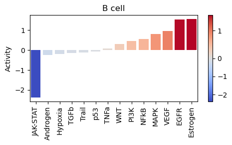
B cell	-0.246842	1.543935	1.558608	-0.183671	-2.382583	0.810554	0.546738	0.451384	-0.143148	0.073370	-0.112629	0.952661	0.301521	-0.070714
Endothelial cell	0.265883	-1.505292	-0.321566	-0.994649	-0.125569	-1.122115	-0.584029	0.969558	1.325543	-0.051087	-0.217974	-1.351533	-0.744210	-1.603530
Epithelial cell	-0.066642	0.350913	0.609130	-0.638363	-2.157498	1.037603	1.325603	-0.099008	0.982241	1.344078	-0.287075	-0.267846	0.073246	-1.125983
Macrophage/Monocyte	0.324897	0.053649	1.877761	-0.324897	-2.601908	0.518574	1.292100	-0.084467	0.196897	0.117583	-0.141024	-0.004292	-0.121309	-0.324401
Mast cell	0.454180	2.103930	0.520413	-0.245265	-1.853323	0.797029	1.094156	0.280248	0.937557	1.111588	0.062696	-0.043590	0.334270	-0.055096
NK cell	0.212747	1.816607	0.449081	-0.603643	-2.053647	0.235018	-0.369732	1.132183	1.386292	-0.611621	-0.477229	0.553257	-0.223066	0.540776
Neutrophils	-0.182056	0.331990	0.078026	-1.963086	-1.363948	-0.124623	-1.486473	-0.260542	-0.215657	-0.964152	1.542883	-0.581928	-0.332444	-0.716360
Plasma cell	-0.350442	0.988855	0.659004	-0.224818	-1.616886	0.544039	2.189130	0.371615	1.108352	0.892480	0.139872	0.120283	0.825329	0.190010
Stromal	0.019815	0.576191	-0.330965	-1.326875	-1.581439	0.551950	1.604827	1.602388	-1.025598	0.574834	0.278758	0.456741	-0.604357	-0.569790
T cell	0.173866	-0.164334	2.026978	-0.180541	-2.333157	0.458294	-0.072737	-0.640231	0.455387	-0.622412	-0.121731	0.468706	-0.874931	-0.989860
cDC	0.667159	0.707137	-0.197105	-1.463723	-1.242213	0.455950	1.736791	1.035391	-0.004090	1.459614	0.176106	1.096091	-0.306651	0.045747

Generate per cell type pathway activity barplots. We use the decoupler plot_barplot function for plotting the pathway activities of each celltype and save the result in png, pdf, svg format.

# show maximum n plots in notebook, all are saved as files
show_n = 2

for contrast in contrasts:
    print(contrast["name"])

    with plt.ioff():
        p_count = 0

        for ct in contrast["cell_types"]:
            bp = dc.plot_barplot(
                contrast["pathway_acts"],
                ct,
                top=25,
                vertical=False,
                return_fig=True,
                figsize=[5, 3],
            )
            plt.title(ct)
            plt.tight_layout()

            if bp is not None:
                ct_fname = ct.replace(" ", "_").replace("/", "_")
                aps.pl.save_fig_mfmt(
                    bp,
                    res_dir=f"{contrast['res_dir']}/pathways/",
                    filename=f"{contrast['name']}_pw_acts_barplot_{ct_fname}",
                    fmt="all",
                )
                # Only show the first two plots in the notebook
                p_count += 1
                if p_count <= show_n:
                    display(bp)
                else:
                    print(f"Not showing: {ct}")

                plt.close()
            else:
                print("No plot for: " + contrast["name"] + ":" + ct)

    print(f"\nResults stored in: {contrast['res_dir']}/pathways")

LUAD_vs_LUSC
Not showing: Epithelial cell
Not showing: Macrophage/Monocyte
Not showing: Mast cell
Not showing: Plasma cell
Not showing: cDC
Not showing: Stromal
Not showing: NK cell
Not showing: Endothelial cell
Not showing: Neutrophils

Results stored in: ../../data/results/10_functional_analysis/LUAD_vs_LUSC/pathways

../_images/1c77c9f5f8a6d3e663db8f07dd4bfb0339086ab777bece40ed8c1f1ba80bd2d8.png

../_images/7b8c34267b3232af935157d58560ab2c2b1ddbc18b1b9f6cdabf6745b8272827.png

Generate pathway activity heatmap#

We use the seaborn clustermap function to generate a clustered heatmap of the celltype pathway activities and save the result in png, pdf, svg format.
Signigficant activity differences are marked with “●”

# generate heatmap plot
for contrast in contrasts:
    # mark significant activities
    sig_mat = np.where(contrast["pathway_pvals"] < 0.05, "●", "")

    with plt.rc_context({"figure.figsize": (5.2, 5)}):
        chm = sns.clustermap(
            contrast["pathway_acts"],
            annot=sig_mat,
            annot_kws={"fontsize": 12},
            center=0,
            cmap="bwr",
            linewidth=0.5,
            cbar_kws={"label": "Pathway activity"},
            vmin=-2,
            vmax=2,
            fmt="s",
            figsize=(7, 7),
        )
        aps.pl.reshape_clustermap(chm, cell_width=0.05, cell_height=0.05)
        aps.pl.save_fig_mfmt(
            chm,
            res_dir=f"{contrast['res_dir']}/pathways/",
            filename=f"{contrast['name']}_pw_acts_heatmap",
            fmt="all",
        )
        plt.show()

        print(f"\nResults stored in: {contrast['res_dir']}/pathways")

../_images/7ae6c53c04cc1915f3f06127d4746ea1f45fd9214de674078da7012fdc95ef9a.png

Results stored in: ../../data/results/10_functional_analysis/LUAD_vs_LUSC/pathways

Generate target gene expression plots for significant pathways#

We genereate expression plots for the target genes of pathways with significant activity differences using the DESeq2 wald statistics (y-axis) and the interaction weight (x-axis).
The results are stored in png, pdf, svg format.

Get significant pathways

# filter for p-value < 0.05
for contrast in contrasts:
    p = contrast["pathway_pvals"]
    sig_pathways_idx = np.where(p < 0.05)

    # make list of celltype / pathway pairs
    sig_pathways = []

    for sig_pw in list(zip(sig_pathways_idx[0], sig_pathways_idx[1])):
        ct = p.index[sig_pw[0]]
        pw = p.columns[sig_pw[1]]
        sig_pathways.append({"ct": ct, "pw": pw})

    contrast["sig_pathways"] = sig_pathways

Generate plot

for contrast in contrasts:
    print(contrast["name"])
    sig_pw = contrast["sig_pathways"]

    # Calculate nrows based on ncol
    n_sig = len(sig_pw)
    ncols = 4 if n_sig >= 4 else n_sig
    nrows = int(np.ceil(n_sig / ncols))

    # Initialize the figure panel
    fig, axs = plt.subplots(nrows=nrows, ncols=ncols, figsize=(ncols * 4, nrows * 4))
    empty_axs = axs.flatten()
    axs = {": ".join(sig_pw.values()): {"ax": ax, "sig_pw": sig_pw} for sig_pw, ax in zip(sig_pathways, axs.flatten())}

    # Run dc.plot_targets for all significant celltype/pathway combinations using the stat values from deseq2
    for key, ax_sig_pw in axs.items():
        dc.plot_targets(
            de_res[ax_sig_pw["sig_pw"]["ct"]].set_index("gene_id"),
            stat="stat",
            source_name=ax_sig_pw["sig_pw"]["pw"],
            net=pwnet,
            top=15,
            return_fig=False,
            ax=ax_sig_pw["ax"],
        )
        ax_sig_pw["ax"].set_title(key)

    # set empty axes invisible
    for ax in range(len(axs), len(empty_axs)):
        empty_axs[ax].set_visible(False)

    plt.tight_layout()
    plt.show()

    # Save figure
    aps.pl.save_fig_mfmt(
        fig,
        res_dir=f"{contrast['res_dir']}/pathways/",
        filename=f"{contrast['name']}_pw_target_expression",
        fmt="all",
    )

    print(f"\nResults stored in: {contrast['res_dir']}/pathways")

LUAD_vs_LUSC

Results stored in: ../../data/results/10_functional_analysis/LUAD_vs_LUSC/pathways

../_images/f6a671b59f0bd9aea7c3dde3f2df5b5de7e82c37bd8cd81957d441023edc0f30.png

Save pathway activity and p-values matrix#

Finally we store the pathway activity scores and p-values in tsv format.

# save tsv
for contrast in contrasts:
    tsv_dir = Path(contrast["res_dir"], "pathways", "tsv")
    os.makedirs(tsv_dir, mode=0o750, exist_ok=True)
    contrast["pathway_acts"].to_csv(f"{tsv_dir}/{contrast['name']}_pathway_acts.tsv", sep="\t")
    contrast["pathway_pvals"].to_csv(f"{tsv_dir}/{contrast['name']}_pathway_pvals.tsv", sep="\t")

6. Infer transcription factor activities with consensus#

Run decoupler consensus method to infer transcription factor activities from the DESeq2 result using the DoRothEA models.
We use the obtained gene level wald statistics stored in stat.

# Infer transcription factor activities with consensus
for contrast in contrasts:
    print(contrast["name"])

    tf_acts, tf_pvals = dc.run_consensus(mat=contrast["stat_mat"], net=tfnet)
    contrast["tf_acts"] = tf_acts
    contrast["tf_pvals"] = tf_pvals
    display(tf_acts)

LUAD_vs_LUSC

	AHR	AR	ARID2	ARID3A	ARNT	ASCL1	ATF1	ATF2	ATF3	ATF4	...	ZNF217	ZNF24	ZNF263	ZNF274	ZNF384	ZNF584	ZNF592	ZNF639	ZNF644	ZNF740
B cell	0.494807	-1.295858	0.635201	1.418887	-0.102753	0.079330	0.869259	0.407446	-0.171582	0.054380	...	0.229161	-0.500840	1.000174	0.400323	0.144617	-0.803723	0.255080	1.367018	0.479102	1.965369
Endothelial cell	-0.549029	-0.115354	-1.938669	0.377054	-0.778608	-0.846926	0.242634	-0.825719	0.402927	-0.937720	...	-1.901210	0.404682	1.336712	-1.310806	-0.052659	-0.974487	-0.098543	0.103671	-0.702017	-0.527577
Epithelial cell	0.799596	0.889566	0.614851	0.587870	-0.160494	-0.669058	1.918827	0.276528	1.026194	0.012645	...	1.058468	-1.142710	0.498509	0.835900	1.142901	-0.769006	-0.369195	0.748939	1.047694	-0.379316
Macrophage/Monocyte	0.658651	-0.061280	1.031650	1.948800	0.418176	0.480713	0.321043	1.301374	0.682867	0.072852	...	1.074232	-0.619390	0.412382	0.137358	0.958108	-0.207613	-1.124615	1.058357	0.958553	0.117008
Mast cell	0.018299	-0.362015	0.351705	1.298517	0.790628	-0.003134	0.310598	2.014740	0.951946	1.399003	...	0.150157	0.076853	1.082928	-0.271137	0.011567	-0.143134	-0.905225	1.381839	-0.294005	0.037592
NK cell	-0.270554	-0.804563	0.147967	0.468447	0.112974	1.337718	0.070423	-0.739791	-0.257967	0.064888	...	1.040004	0.472885	2.216979	0.026001	0.443216	0.484252	0.911763	1.514379	0.654045	2.159696
Neutrophils	0.042768	-1.624405	0.320883	-0.345890	-0.638695	0.249693	-0.880325	-1.321099	0.296990	-1.317136	...	-0.538398	0.529491	0.347337	-0.747914	-1.146214	-0.443622	-0.138553	-0.401604	0.452665	-0.298905
Plasma cell	-0.316239	-0.512138	1.408229	0.054453	0.374180	0.277874	0.389478	2.105656	1.677759	2.472244	...	-0.287736	-0.923191	0.389007	-0.030057	-0.093641	0.177626	1.005671	2.013895	0.280040	0.210682
Stromal	-0.199434	-1.809133	0.299511	0.631933	1.150876	0.046605	-0.558228	-0.047530	-0.146499	1.124004	...	-1.005617	-0.213832	1.378833	1.708247	-1.704742	-0.277866	-1.160813	-0.935735	-0.460369	-0.501042
T cell	1.016850	-1.446534	1.498921	1.636793	-0.205554	-0.167935	0.127256	-0.304119	0.396686	0.616725	...	0.362580	0.122930	0.173679	0.914766	1.057778	0.622133	1.063043	1.867057	0.635081	1.690971
cDC	0.952299	-0.233353	0.193726	-0.543061	-0.542293	-0.360546	0.758699	1.044606	0.465229	0.867267	...	0.528510	0.563882	0.865910	0.903282	0.332664	0.016136	0.856794	0.305656	0.244124	-1.040939

11 rows × 297 columns

Generate per cell type transcription factor activity barplots#

We use the decoupler plot_barplot function for plotting the transcription factor activities of each celltype and save the result in png, pdf, svg format.

# show maximum n plots in notebook, all are saved as files
show_n = 2

for contrast in contrasts:
    print(contrast["name"])

    with plt.ioff():
        p_count = 0

        for ct in contrast["cell_types"]:
            bp = dc.plot_barplot(
                contrast["tf_acts"],
                ct,
                top=25,
                vertical=False,
                return_fig=True,
                figsize=[5, 3],
            )
            plt.title(ct)
            plt.tight_layout()

            if bp is not None:
                ct_fname = ct.replace(" ", "_").replace("/", "_")
                aps.pl.save_fig_mfmt(
                    bp,
                    res_dir=f"{contrast['res_dir']}/transcription_factors/",
                    filename=f"{contrast['name']}_tf_acts_barplot_{ct_fname}",
                    fmt="all",
                )

                # Only show the first two plots in the notebook
                p_count += 1
                if p_count <= show_n:
                    display(bp)
                else:
                    print(f"Not showing: {ct}")

                plt.close()

            else:
                print("No plot for: " + contrast["name"] + ":" + ct)

        print(f"\nResults stored in: {contrast['res_dir']}/transcription_factors")

LUAD_vs_LUSC
Not showing: Epithelial cell
Not showing: Macrophage/Monocyte
Not showing: Mast cell
Not showing: Plasma cell
Not showing: cDC
Not showing: Stromal
Not showing: NK cell
Not showing: Endothelial cell
Not showing: Neutrophils

Results stored in: ../../data/results/10_functional_analysis/LUAD_vs_LUSC/transcription_factors

../_images/9caf2fe1640f8c32a609aa3bf17512e9fde0a174abfc2bc6aa6b2f42ccf456b2.png

../_images/925b8c0fbe907b40272e1552ca162cdc90fc86584ba6fe65cf13c03424aff583.png

Generate transcription factor activity heatmap#

We use the seaborn clustermap function to generate a clustered heatmap of the celltype transcription factor activities and save the result in png, pdf, svg format.
Signigficant activity differences are marked with “●”

# generate heatmap plot
for contrast in contrasts:
    # get acts and pvals
    pvals = contrast["tf_pvals"].copy()
    acts = contrast["tf_acts"].copy()

    # select the columns that have significant acts (pval < 0.05)
    sig_pval_cols = pvals.columns[(pvals < 0.05).any()]

    pvals = pvals[sig_pval_cols]
    acts = acts[sig_pval_cols]

    # mark significant activities
    sig_mat = np.where(pvals < 0.05, "●", "")

    with plt.rc_context({"figure.figsize": (10, 5)}):
        chm = sns.clustermap(
            acts,
            annot=sig_mat,
            annot_kws={"fontsize": 10},
            center=0,
            cmap="bwr",
            linewidth=0.5,
            cbar_kws={"label": "TF activity"},
            vmin=-2,
            vmax=2,
            fmt="s",
            xticklabels=True,
            figsize=(4.5, 4.5),
        )
        aps.pl.reshape_clustermap(chm, cell_width=0.05, cell_height=0.05)
        aps.pl.save_fig_mfmt(
            chm,
            res_dir=f"{contrast['res_dir']}/transcription_factors/",
            filename=f"{contrast['name']}_tf_acts_heatmap",
            fmt="all",
        )
        plt.tight_layout()
        plt.show()

    print(f"\nResults stored in: {contrast['res_dir']}/transcription_factors")

../_images/d5de2d396c4869c5d6da919efd6c486b1514160776d40eb35201f0f2dab0a9b5.png

Results stored in: ../../data/results/10_functional_analysis/LUAD_vs_LUSC/transcription_factors

Volcano plots of expression of target genes from transcription factors of interest#

We genereate volcano plots for the target genes of selected transcription factors with significant activity differences using the DESeq2 log2foldChange (x-axis) and padj (y-axis) values.
For each transcription factor of interest a panel of celltype specific volcano plots will be created. The results are stored in png, pdf, svg format.

tf_of_interest: List of transcription factors in which we are interested and for whose target genes we want to generate a volcano plot

# Define transcription factors of interest
tf_of_interest = ["CEBPA", "SOX13", "SPI1"]

for contrast in contrasts:
    # Extract logFCs and pvals
    logFCs = contrast["lfc_mat"]
    pvals = contrast["fdr_mat"]
    tf_pvals = contrast["tf_pvals"]

    # get sig ct for tfoi
    n_sig = 0
    sig_tf = {}
    for ct in contrast["cell_types"]:
        for tfoi in tf_of_interest:
            if tf_pvals.loc[ct][tfoi] < 0.05:
                if tfoi not in sig_tf:
                    sig_tf[tfoi] = []
                sig_tf[tfoi].append({"ct": ct, "tf": tfoi})
                n_sig += 1

    # generate a volcano plot panel for each transcription factor of interest:
    # the panels show volcano plots for each celltype in which there is a
    # signigicant transcription factor activity
    for tf in sig_tf.keys():
        n_sig = len(sig_tf[tf])

        # Calculate nrows based on ncol
        ncols = 4 if n_sig >= 4 else n_sig
        nrows = int(np.ceil(n_sig / ncols))

        # Initialize the figure panel
        fig, axs = plt.subplots(nrows=nrows, ncols=ncols, figsize=(ncols * 4, nrows * 4))
        empty_axs = axs.flatten()
        axs = [{"ct_tf": ct_tf, "ax": ax} for ct_tf, ax in zip(sig_tf[tf], axs.flatten())]

        for ax in axs:
            dc.plot_volcano(
                logFCs,
                pvals,
                ax["ct_tf"]["ct"],
                name=ax["ct_tf"]["tf"],
                net=tfnet,
                top=10,
                sign_thr=0.1,
                lFCs_thr=0.5,
                return_fig=False,
                ax=ax["ax"],
            )

        # set empty axes invisible
        for ax in range(len(axs), len(empty_axs)):
            empty_axs[ax].set_visible(False)

        plt.tight_layout()
        plt.show()

        # Save figure
        aps.pl.save_fig_mfmt(
            fig,
            res_dir=f"{contrast['res_dir']}/transcription_factors/",
            filename=f"{contrast['name']}_{tf}_target_expression",
            fmt="all",
        )

    print(f"\nResults stored in: {contrast['res_dir']}/transcription_factors")

../_images/4699ae3f63ccdb2712e3b5732228e82b86e30d8b2bed4c7a57180e2817f623ff.png

../_images/27f50892fb6f74782919865c00daefde1042ee65f3cc233dc7a96aa1ca9a57fd.png

../_images/abbbef9e729891e007bac20476f36520d1ed11d7874fbf113fc0f91378b2ff2c.png

Results stored in: ../../data/results/10_functional_analysis/LUAD_vs_LUSC/transcription_factors

Save transcription factor activity and p-values matrix#

Finally we store the transcription factor activity scores and p-values in tsv format.

# save tsv
for contrast in contrasts:
    tsv_dir = Path(contrast["res_dir"], "transcription_factors", "tsv")
    os.makedirs(tsv_dir, mode=0o750, exist_ok=True)
    contrast["tf_acts"].to_csv(f"{tsv_dir}/{contrast['name']}_transcription_factor_acts.tsv", sep="\t")
    contrast["tf_pvals"].to_csv(f"{tsv_dir}/{contrast['name']}_transcription_factor_pvals.tsv", sep="\t")

7. Infer enrichment of biological terms with GSEA using significant differential expressed genes#

We can utilize MSigDB to assign biological terms to the differentially expressed genes. In this case, we will employ the run_gsea method from decoupler.

Run GSEA#

We use the wald statistics (stat) from the DESeq2 result to rank the genes.

for contrast in contrasts:
    # run_gsea from decoupler
    gsea_estimate, gsea_norm, gsea_pvals = dc.run_gsea(
        contrast["stat_mat"],
        msigdb,
        source="geneset",
        target="genesymbol",
        times=1000,
        batch_size=10000,
        min_n=5,
        seed=4711,
        verbose=False,
    )

    contrast["gsea_estimate"] = gsea_estimate
    contrast["gsea_norm"] = gsea_norm
    contrast["gsea_pvals"] = gsea_pvals

Now we correct for multiple hypothesis testing using BH

for contrast in contrasts:
    # make long format
    gsea_pvals = contrast["gsea_pvals"]
    gsea_pvals_long = pd.melt(
        gsea_pvals.T.rename_axis("source").reset_index(),
        id_vars=["source"],
        var_name="cell_type",
        value_name="pval",
    )

    # run fdrcorrection and add padj to df
    gsea_pvals_long["padj"] = statsmodels.stats.multitest.fdrcorrection(gsea_pvals_long["pval"].values)[1]

    # make padj_mat
    gsea_padj = gsea_pvals_long.pivot(index="cell_type", columns="source", values="padj")
    gsea_padj.index.name = None

    # store the padj for the contrast and make sure that we preserve the order of row and columns
    contrast["gsea_padj"] = gsea_padj.reindex(index=contrast["gsea_pvals"].index).reindex(
        contrast["gsea_pvals"].columns, axis=1
    )

Generate MSigDB heatmap from GSEA normalized enrichment scores#

We use the seaborn heatmap function to generate a heatmap of the biological terms assigned by GSEA to the different celltypes and save the result in png, pdf, svg format.
Signigficantly overrepresented terms are marked with “●”

NES (normalized enrichment score) is color-coded

# Plot heatmap of GSEA result
for contrast in contrasts:
    gsea_padj = contrast["gsea_padj"]

    gsea_norm = contrast["gsea_norm"].copy()

    # filter for enriched (positve nes score)
    gsea_norm[gsea_norm < 0] = 0

    # mark significant enrichment
    sig_mat = np.where(gsea_padj[gsea_norm > 0] < 0.05, "●", "")

    # create figure
    fig, ax = plt.subplots(nrows=1, ncols=1, figsize=(17, 10))

    # create heatmap
    hm = sns.heatmap(
        gsea_norm,
        annot=sig_mat,
        robust=True,
        cmap="viridis",
        linewidth=0.5,
        cbar=True,
        cbar_kws={"label": "normalized enrichment score", "shrink": 0.4},
        fmt="s",
        square=True,
        xticklabels=True,
        ax=ax,
    )
    plt.tight_layout()
    aps.pl.save_fig_mfmt(
        fig,
        res_dir=f"{contrast['res_dir']}/MSigDB/",
        filename=f"{contrast['name']}_MSigDB_GSEA_heatmap",
        fmt="all",
    )
    plt.show()

    print(f"\nResults stored in: {contrast['res_dir']}/MSigDB")

../_images/d2146bd27855052cdd6a4a877bb24391567a856fb30b8c2ddf8142f172880264.png

Results stored in: ../../data/results/10_functional_analysis/LUAD_vs_LUSC/MSigDB

Visualize the most enriched terms as barplot#

We use the decoupler plot_barplot function to generate barplots of the most enriched biological and save the result in png, pdf, svg format.

top_n: top n cell types to generate barplots for. Cell types are sorted by the highest GSEA score

top_n = 4

# show top n celltypes
for contrast in contrasts:
    print(contrast["name"] + "\n")
    display(np.min(contrast["gsea_padj"].T, axis=0).sort_values().head(top_n))

LUAD_vs_LUSC

B cell             9.453365e-14
Neutrophils        6.443057e-11
Epithelial cell    2.340751e-10
Mast cell          5.205902e-09
dtype: float64

for contrast in contrasts:
    gsea_norm = contrast["gsea_norm"].copy()

    # filter for enriched (positve nes score)
    gsea_norm[gsea_norm < 0] = 0

    # get top n celltypes
    top_celltypes = np.min(gsea_padj.T, axis=0).sort_values().head(top_n).index.values

    with plt.rc_context({"figure.figsize": (8, 3)}):
        for ct in top_celltypes:
            vcenter = np.max(gsea_norm.T[ct]) / 2
            bp = dc.plot_barplot(
                gsea_norm,
                ct,
                top=10,
                vertical=True,
                return_fig=True,
                vmin=0,
                vcenter=vcenter,
                cmap="Reds",
                figsize=[8, 3],
            )
            plt.title(ct)
            plt.xlabel("normalized enrichment score")
            plt.tight_layout()
            plt.show()

            if bp is not None:
                ct_fname = ct.replace(" ", "_").replace("/", "_")
                aps.pl.save_fig_mfmt(
                    bp,
                    res_dir=f"{contrast['res_dir']}/MSigDB/",
                    filename=f"{contrast['name']}_top_terms_barplot_{ct_fname}",
                    fmt="all",
                )
            else:
                print("No plot for: " + contrast["name"] + ":" + ct)
    plt.close()

    print(f"\nResults stored in: {contrast['res_dir']}/MSigDB")

../_images/6dd040aebf221dc930b4dc0e99e92d39fc06d998a16afa142fe70e30fae96db9.png

../_images/2fcf6ab82763d1b7e00528dbbc1e2cf5b6b501d19f297fa3168750ee94024c2c.png

../_images/e6c00daf9af3d49701b90b0a10221497b84583cbc6f4d0c3038f9de8391cfd29.png

../_images/bffb403c7da1585847c1e35fd5715dcd6a9d05c6a7e68aec86c3530617169601.png

Results stored in: ../../data/results/10_functional_analysis/LUAD_vs_LUSC/MSigDB

Generate volcano plots for the most enriched term of the top n celltypes#

top_n: number of celltypes to generate volcano plot of the most enriched term

top_n = 6

# show top n celltypes
for contrast in contrasts:
    print(contrast["name"] + "\n")
    display(np.min(contrast["gsea_padj"].T, axis=0).sort_values().tail(top_n))

LUAD_vs_LUSC

cDC                 1.483697e-07
Plasma cell         5.775455e-07
Stromal             6.139488e-07
Endothelial cell    3.132816e-06
T cell              6.968669e-06
NK cell             3.174736e-05
dtype: float64

for contrast in contrasts:
    logFC = contrast["lfc_mat"]
    pvals = contrast["fdr_mat"]

    # get top n celltypes
    top_celltypes = np.min(contrast["gsea_padj"].T, axis=0).sort_values().head(top_n).index.values

    # get top term of each celltype
    top_term = {}
    for ct in top_celltypes:
        top_term[ct] = contrast["gsea_norm"].loc[ct].idxmax()

    # Calculate nrows based on ncol
    ncols = 3 if top_n >= 3 else n_sig
    nrows = int(np.ceil(top_n / ncols))

    # Initialize the figure panel
    fig, axs = plt.subplots(nrows=nrows, ncols=ncols, figsize=(ncols * 6, nrows * 4))
    empty_axs = axs.flatten()
    axs = [[{"ct": t, "term": top_term[t]}, ax] for t, ax in zip(top_term, axs.flatten())]

    for t, ax in axs:
        dc.plot_volcano(
            logFCs,
            pvals,
            t["ct"],
            name=t["term"],
            net=msigdb,
            top=10,
            sign_thr=0.1,
            lFCs_thr=0.5,
            source="geneset",
            target="genesymbol",
            weight=None,
            return_fig=False,
            ax=ax,
        )

    # set empty axes invisible
    for ax in range(len(axs), len(empty_axs)):
        empty_axs[ax].set_visible(False)

    plt.tight_layout()
    plt.show()

    # Save figure
    aps.pl.save_fig_mfmt(
        fig,
        res_dir=f"{contrast['res_dir']}/MSigDB/",
        filename=f"{contrast['name']}_top_terms_target_expression",
        fmt="all",
    )

    print(f"\nResults stored in: {contrast['res_dir']}/MSigDB")

../_images/52736057ea9977ddb2382a1a6cc127422453293d16dc9074f8f4ab7246c7e44b.png

Results stored in: ../../data/results/10_functional_analysis/LUAD_vs_LUSC/MSigDB

Save GSEA scores of enriched terms#

Finally we store the GSEA scores of enriched terms in tsv format.

# save tsv
for contrast in contrasts:
    tsv_dir = Path(contrast["res_dir"], "MSigDB", "tsv")
    os.makedirs(tsv_dir, mode=0o750, exist_ok=True)
    contrast["gsea_norm"].to_csv(f"{tsv_dir}/{contrast['name']}_MSigDB_GSEA_nes.tsv", sep="\t")
    contrast["gsea_estimate"].to_csv(f"{tsv_dir}/{contrast['name']}_MSigDB_GSEA_estimate.tsv", sep="\t")
    contrast["gsea_pvals"].to_csv(f"{tsv_dir}/{contrast['name']}_MSigDB_GSEA_pvals.tsv", sep="\t")
    contrast["gsea_padj"].to_csv(f"{tsv_dir}/{contrast['name']}_MSigDB_GSEA_padj.tsv", sep="\t")

8. CytoSig analysis#

We define enriched cytokine signaling signatures in the tumor cells using the CytoSig signature matrix an the decoupler consesus scoring function.

First we reformat the signature matrix into long format

# reformat the signature matrix
cyto_sig = pd.melt(
    cytosig_signature.rename_axis("target").reset_index(),
    var_name="source",
    id_vars=["target"],
    value_name="weight",
).reindex(columns=["source", "target", "weight"])
cyto_sig

	source	target	weight
0	Activin A	A2M	0.050964
1	Activin A	A4GALT	-0.208403
2	Activin A	AAAS	-0.026028
3	Activin A	AACS	-0.107110
4	Activin A	AAK1	-0.022077
...	...	...	...
329761	WNT3A	ZZZ3	0.027164
329762	WNT3A	CHN2	-0.064087
329763	WNT3A	ESRRG	0.042413
329764	WNT3A	FHIT	-0.046138
329765	WNT3A	HOXB6	0.053906

329766 rows × 3 columns

Run the decoupler consensus scoring function using the DESeq2 wald statistics and the CytoSig net

# Infer cytokin signaling with consensus
for contrast in contrasts:
    print(contrast["name"])

    cs_acts, cs_pvals = dc.run_consensus(mat=contrast["stat_mat"], net=cyto_sig)
    contrast["cs_acts"] = cs_acts
    contrast["cs_pvals"] = cs_pvals
    display(cs_acts)

LUAD_vs_LUSC

	Activin A	BDNF	BMP2	BMP4	BMP6	CD40L	CXCL12	EGF	FGF2	GCSF	...	PGE2	TGFA	TGFB1	TGFB2	TGFB3	TNFA	TRAIL	TWEAK	VEGFA	WNT3A
B cell	-0.482646	2.259695	-0.863616	-1.478322	0.045383	-0.587955	-1.131240	0.708744	-2.260390	0.762260	...	0.096722	0.382647	-0.597530	1.654242	-1.672500	0.085604	-0.374362	-0.116501	0.441778	0.904713
Endothelial cell	-0.140653	-1.391896	0.178591	0.526312	1.052298	0.599148	-0.009525	-1.536898	0.367362	0.183483	...	-0.882414	-0.814086	0.080817	-0.311397	0.818801	0.118420	0.831849	-0.907669	-0.890997	1.998671
Epithelial cell	0.272666	0.784764	0.310924	1.235774	-0.914101	1.092303	0.749393	0.998541	0.405041	0.557434	...	1.420431	0.623688	1.169039	0.339757	2.496500	0.739314	0.873977	0.676544	0.679720	0.279122
Macrophage/Monocyte	0.041470	0.338627	0.317325	0.641722	0.309349	1.157407	0.188017	1.147379	0.363295	1.282793	...	0.391389	0.514752	0.716912	0.610758	1.851552	0.948503	0.728291	0.287427	1.120714	0.509945
Mast cell	-0.096104	0.772115	-0.267422	0.273004	-0.017583	1.223186	0.569611	1.404026	0.896434	0.931618	...	0.340526	1.117030	0.683753	0.585125	0.333965	0.926995	1.497205	-0.190361	2.420311	-0.224754
NK cell	0.579675	1.941291	0.323327	-0.651686	0.393145	0.514874	0.541557	0.720228	-1.358832	0.430220	...	1.045958	0.888556	0.256206	0.933542	1.715606	1.100328	0.643063	1.301733	0.427909	0.206403
Neutrophils	-0.142243	-0.284395	-0.146106	0.043163	1.370602	0.466852	-0.735402	-1.045701	0.103361	0.851347	...	0.029674	-0.742348	0.028969	-0.268258	0.710881	-0.522137	1.238972	-0.554146	-0.016647	1.303866
Plasma cell	0.256896	0.878637	0.040202	-0.118374	-0.959249	0.492737	0.818973	1.345826	-0.165030	0.694331	...	0.916952	1.382699	0.226926	1.535075	1.177693	1.292434	0.997565	0.339793	1.494568	0.082868
Stromal	-0.200350	-0.317472	-0.636725	-1.060266	0.785712	1.281654	0.419830	-0.099255	0.321945	0.117448	...	0.444467	-1.360930	-0.758919	-1.296940	-0.953828	0.372752	2.755995	-0.088483	-0.576638	-0.388535
T cell	0.140575	1.639995	-0.324083	-0.616470	-0.592388	0.268146	-0.642872	1.222686	-0.956480	-0.371912	...	0.765180	0.291763	0.594390	1.611180	1.894272	0.106447	0.613308	0.675075	0.567940	0.762486
cDC	-0.167750	-0.032822	0.477761	0.674290	0.665356	2.155193	0.137226	0.423278	-0.292649	0.860476	...	0.159508	0.462986	0.766819	0.040337	1.995206	1.628578	1.295601	0.865028	0.308939	0.840638

11 rows × 51 columns

Generate signaling activity heatmap#

We use the seaborn clustermap function to generate a clustered heatmap of the celltype signaling activities and save the result in png, pdf, svg format.
Signigficant signaling activity differences are marked with “●”

# generate heatmap plot
for contrast in contrasts:
    # get acts and pvals
    pvals = contrast["cs_pvals"].copy()
    acts = contrast["cs_acts"].copy()

    # select the columns that have significant acts (pval < 0.05)
    sig_pval_cols = pvals.columns[(pvals < 0.05).any()]

    pvals = pvals[sig_pval_cols]
    acts = acts[sig_pval_cols]

    # mark significant activities
    sig_mat = np.where(pvals < 0.05, "●", "")

    with plt.rc_context({"figure.figsize": (10, 10)}):
        chm = sns.clustermap(
            acts,
            annot=sig_mat,
            annot_kws={"fontsize": 10},
            center=0,
            cmap="bwr",
            linewidth=0.5,
            cbar_kws={"label": "signaling activity"},
            vmin=-2,
            vmax=2,
            fmt="s",
            xticklabels=True,
            figsize=(6, 6),
        )
        aps.pl.reshape_clustermap(chm, cell_width=0.05, cell_height=0.05)
        aps.pl.save_fig_mfmt(
            chm,
            res_dir=f"{contrast['res_dir']}/cytokine_signaling/",
            filename=f"{contrast['name']}_signaling_heatmap",
            fmt="all",
        )
        plt.show()

        print(f"\nResults stored in: {contrast['res_dir']}/cytokine_signaling")

../_images/81dd2e5940643ea379c34aaebb8d481e890e41e3090a01a28a008bd2e3e7a5af.png

Results stored in: ../../data/results/10_functional_analysis/LUAD_vs_LUSC/cytokine_signaling

Save cytokine signaling activity scores and p-values matrix#

Finally we store the cytokine signaling activity scores and p-values in tsv format.

# save tsv
for contrast in contrasts:
    tsv_dir = Path(contrast["res_dir"], "cytokine_signaling", "tsv")
    os.makedirs(tsv_dir, mode=0o750, exist_ok=True)
    contrast["cs_acts"].to_csv(f"{tsv_dir}/{contrast['name']}_CytoSig_acts.tsv", sep="\t")
    contrast["cs_pvals"].to_csv(f"{tsv_dir}/{contrast['name']}_CytoSig_pvals.tsv", sep="\t")

Functional analysis: PROGENy / DoRothEA / CytoSig

Contents

Functional analysis: PROGENy / DoRothEA / CytoSig#

1. Configure paths#

2. Load data#

3. Define contrasts#

4. Read DESeq2 results#

5. Infer pathway activities with consensus#

Generate pathway activity heatmap#

Generate target gene expression plots for significant pathways#

Save pathway activity and p-values matrix#

6. Infer transcription factor activities with consensus#

Generate per cell type transcription factor activity barplots#

Generate transcription factor activity heatmap#

Volcano plots of expression of target genes from transcription factors of interest#

Save transcription factor activity and p-values matrix#

7. Infer enrichment of biological terms with GSEA using significant differential expressed genes#

Run GSEA#

Generate MSigDB heatmap from GSEA normalized enrichment scores#

Visualize the most enriched terms as barplot#

Generate volcano plots for the most enriched term of the top n celltypes#

Save GSEA scores of enriched terms#

8. CytoSig analysis#

Generate signaling activity heatmap#

Save cytokine signaling activity scores and p-values matrix#