Differential gene expression#
One of the most commonly asked questions when comparing between conditions is which genes are differentially expressed. In statistical terms, we ask if the mean gene expression differs between two groups more than what would be expected by random chance. A common fallacy here is that frequently applied statistical tests assume independence of the observations, while cells from the same sample or patient are not independent. This is also called “pseudoreplication bias” and leads to drastically inflated p-values [Squair et al., 2021, Zimmerman et al., 2021].
Unfortunately, the differential testing
functions available from the most commonly used frameworks (e.g. scanpy.tl.rank_genes_groups() in scanpy) do not account for this, allowing for qualitative comparisons at best. As an alternative, Squair et al. [2021] suggest to aggregate samples into “pseudo-bulks” and apply tools originally designed for comparing bulk RNA-seq samples.
In this section, we are going to demonstrate how to generate pseudo-bulk samples by cell-type using decoupler [Badia-i-Mompel et al., 2022] and apply DESeq2 [Love et al., 2014] to perform cell-type-specific comparison between conditions.
See also
The Differential gene expression chapter of the single-cell best practice book [Heumos et al., 2023].
1.Load libraries#
%load_ext autoreload
%autoreload 2
import re
import subprocess as sp
from pathlib import Path

import decoupler as dc
import matplotlib.pyplot as plt
import pandas as pd
import scanpy as sc
from anndata import AnnData
from tqdm.contrib.concurrent import process_map

import atlas_protocol_scripts as aps
2. Load input data#
Load the annotated AnnData object
adata_path = "../../data/input_data_zenodo/atlas-integrated-annotated.h5ad"
adata = sc.read_h5ad(adata_path)
Define the paths to the scripts for DESeq2. The script is shipped as part of the
atlas_protocolrepo.
deseq_script_path = "../../bin/deseq2.R"
Create output directories
deseq_results = Path("../../data/results/differential_expression/")
!mkdir -p {deseq_results}
3. Generate Pseudobulk#
Here, we aggregate counts by biological replicate (patient) for each cell-type individually.
subset AnnData to the cells of interest. In this case, we only focus on cells originating from primary tumor samples and the two conditions (LUAD vs. LUSC) we are going to compare.
adata = adata[adata.obs["origin"].isin(["tumor_primary"]) & adata.obs["condition"].isin(["LUAD", "LUSC"])]
adata
View of AnnData object with n_obs × n_vars = 25892 × 17837
    obs: 'sample', 'uicc_stage', 'sex', 'ever_smoker', 'driver_genes', 'condition', 'age', 'patient', 'tissue', 'origin', 'dataset', 'cell_type', 'cell_type_predicted', 'doublet_status', 'leiden', 'n_genes_by_counts', 'total_counts', 'total_counts_mito', 'pct_counts_mito', 'cell_type_coarse', 'cell_type_tumor', 'tumor_stage', 'EGFR_mutation', 'TP53_mutation', 'ALK_mutation', 'BRAF_mutation', 'ERBB2_mutation', 'KRAS_mutation', 'ROS_mutation', 'origin_fine', 'study', 'platform', 'platform_fine', 'cell_type_major', 'batch', '_predictions', '_leiden', '_cell_type_tumor_predicted'
    var: 'is_highly_variable', 'mito', 'n_cells_by_counts', 'mean_counts', 'pct_dropout_by_counts', 'total_counts'
    uns: '_cell_type_tumor_predicted_colors', '_scvi', 'cell_type_coarse_colors', 'cell_type_colors', 'cell_type_major_colors', 'cell_type_predicted_colors', 'cell_type_tumor_colors', 'condition_colors', 'dataset_colors', 'doublet_status_colors', 'ever_smoker_colors', 'hvg', 'leiden_colors', 'neighbors', 'origin_colors', 'platform_colors', 'sex_colors', 'tumor_stage_colors', 'uicc_stage_colors', 'umap'
    obsm: 'X_scANVI', 'X_scVI', 'X_umap'
    layers: 'raw_counts'
    obsp: 'connectivities', 'distances'
Generate pseudobulk
Important
Generate pseudo-bulk based on raw counts and aggregate them by summing up.
# Get pseudo-bulk profile
pdata = dc.get_pseudobulk(
    adata,
    sample_col="sample",
    groups_col=["cell_type_coarse", "condition"],
    layer="raw_counts",  # layer where raw counts are store in adata
    mode="sum",
    min_cells=0,  # we are setting this to 0 and filter in an explicit, separate step.
    min_counts=0,
)
pdata
AnnData object with n_obs × n_vars = 223 × 17837
    obs: 'sample', 'uicc_stage', 'sex', 'ever_smoker', 'driver_genes', 'condition', 'age', 'patient', 'tissue', 'origin', 'dataset', 'doublet_status', 'total_counts_mito', 'pct_counts_mito', 'cell_type_coarse', 'tumor_stage', 'EGFR_mutation', 'TP53_mutation', 'ALK_mutation', 'BRAF_mutation', 'ERBB2_mutation', 'KRAS_mutation', 'ROS_mutation', 'origin_fine', 'study', 'platform', 'platform_fine', 'batch', '_predictions', '_leiden', '_cell_type_tumor_predicted', 'cell_type_coarse_condition', 'psbulk_n_cells', 'psbulk_counts'
    layers: 'psbulk_props'
Inspect the table of “pseudobulk samples”
pdata.obs
| sample | uicc_stage | sex | ever_smoker | driver_genes | condition | age | patient | tissue | origin | ... | study | platform | platform_fine | batch | _predictions | _leiden | _cell_type_tumor_predicted | cell_type_coarse_condition | psbulk_n_cells | psbulk_counts | |
|---|---|---|---|---|---|---|---|---|---|---|---|---|---|---|---|---|---|---|---|---|---|
| Lambrechts_Thienpont_2018_6653_scrBT1430m_B cell_LUAD | Lambrechts_Thienpont_2018_6653_scrBT1430m | III | male | yes | NaN | LUAD | 65.0 | Lambrechts_Thienpont_2018_6653_6 | lung | tumor_primary | ... | Lambrechts_Thienpont_2018 | 10x | 10x_3p_v2 | NaN | NaN | NaN | NaN | B cell_LUAD | 178.0 | 8.976160e+05 |
| Lambrechts_Thienpont_2018_6653_scrBT1431m_B cell_LUAD | Lambrechts_Thienpont_2018_6653_scrBT1431m | III | male | yes | NaN | LUAD | 65.0 | Lambrechts_Thienpont_2018_6653_6 | lung | tumor_primary | ... | Lambrechts_Thienpont_2018 | 10x | 10x_3p_v2 | NaN | NaN | NaN | NaN | B cell_LUAD | 702.0 | 3.154887e+06 |
| Lambrechts_Thienpont_2018_6653_scrBT1432m_B cell_LUAD | Lambrechts_Thienpont_2018_6653_scrBT1432m | III | male | yes | NaN | LUAD | 65.0 | Lambrechts_Thienpont_2018_6653_6 | lung | tumor_primary | ... | Lambrechts_Thienpont_2018 | 10x | 10x_3p_v2 | NaN | NaN | NaN | NaN | B cell_LUAD | 114.0 | 5.869860e+05 |
| Maynard_Bivona_2020_LT_S42_B cell_LUAD | Maynard_Bivona_2020_LT_S42 | IV | female | no | EGFR | LUAD | 56.0 | Maynard_Bivona_2020_TH158 | lung | tumor_primary | ... | Maynard_Bivona_2020 | Smart-seq2 | Smart-seq2 | NaN | NaN | NaN | NaN | B cell_LUAD | 10.0 | 5.065048e+07 |
| Maynard_Bivona_2020_LT_S56_B cell_LUAD | Maynard_Bivona_2020_LT_S56 | IV | male | no | ALK | LUAD | 37.0 | Maynard_Bivona_2020_TH231 | lung | tumor_primary | ... | Maynard_Bivona_2020 | Smart-seq2 | Smart-seq2 | NaN | NaN | NaN | NaN | B cell_LUAD | 2.0 | 1.941628e+06 |
| ... | ... | ... | ... | ... | ... | ... | ... | ... | ... | ... | ... | ... | ... | ... | ... | ... | ... | ... | ... | ... | ... |
| UKIM-V_P1_tumor_primary_pDC_LUAD | UKIM-V_P1_tumor_primary | I | female | yes | NaN | LUAD | 65.0 | UKIM-V_P1 | lung | tumor_primary | ... | UKIM-V | BD-Rhapsody | BD-Rhapsody | NaN | NaN | NaN | NaN | pDC_LUAD | 25.0 | 8.279220e+05 |
| UKIM-V_P3_tumor_primary_pDC_LUAD | UKIM-V_P3_tumor_primary | I | male | yes | NaN | LUAD | 64.0 | UKIM-V_P3 | lung | tumor_primary | ... | UKIM-V | BD-Rhapsody | BD-Rhapsody | NaN | NaN | NaN | NaN | pDC_LUAD | 15.0 | 1.456810e+05 |
| Lambrechts_Thienpont_2018_6653_BT1375_pDC_LUSC | Lambrechts_Thienpont_2018_6653_BT1375 | I | male | yes | NaN | LUSC | 60.0 | Lambrechts_Thienpont_2018_6653_7 | lung | tumor_primary | ... | Lambrechts_Thienpont_2018 | 10x | 10x_3p_v2 | NaN | NaN | NaN | NaN | pDC_LUSC | 3.0 | 6.947000e+03 |
| Lambrechts_Thienpont_2018_6653_BT1377_pDC_LUSC | Lambrechts_Thienpont_2018_6653_BT1377 | I | male | yes | NaN | LUSC | 60.0 | Lambrechts_Thienpont_2018_6653_7 | lung | tumor_primary | ... | Lambrechts_Thienpont_2018 | 10x | 10x_3p_v2 | NaN | NaN | NaN | NaN | pDC_LUSC | 1.0 | 6.048000e+03 |
| UKIM-V_P2_tumor_primary_pDC_LUSC | UKIM-V_P2_tumor_primary | I | female | yes | NaN | LUSC | 70.0 | UKIM-V_P2 | lung | tumor_primary | ... | UKIM-V | BD-Rhapsody | BD-Rhapsody | NaN | NaN | NaN | NaN | pDC_LUSC | 8.0 | 1.085030e+05 |
223 rows × 34 columns
4. Filter samples#
In this step, we are removing samples that consist of too few cells or have a small number of total counts in both conditions.
Plot relationship of counts and cells per dataset and cell-type
for col in ["dataset", "cell_type_coarse", "condition"]:
    dc.plot_psbulk_samples(pdata, groupby=col, figsize=(3, 3))


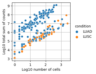
Remove samples with less than 10 cells or less than 1000 counts
pdata = pdata[(pdata.obs["psbulk_n_cells"] >= 10) & (pdata.obs["psbulk_counts"] >= 1000)]
5. Split pseudobulk by cell-type#
For the following steps, we treat each cell-type separately, therefore we split the pseudobulk object into a dictionary of objects per cell-type.
Define list of cell-types
cell_types = pdata.obs["cell_type_coarse"].unique()
Generate per-cell-type dictionary
pdata_by_cell_type = {}
for ct in cell_types:
    pb = pdata[pdata.obs["cell_type_coarse"] == ct, :].copy()
    if pb.obs["condition"].nunique() <= 1:
        print(f"Cell type {ct} does not have samples in all groups")
    else:
        pdata_by_cell_type[ct] = pb
Cell type pDC does not have samples in all groups
6. Filter genes#
Here, we filter noisy genes with a low expression value. We remove genes that do not have a certain number of total counts (min_total_count) and have a minimum number of counts in at least \(n\) samples, where \(n\) equals to the number of samples
in the smallest group (or less, if there is a sufficient number of samples).
This needs to be done for each cell-type individually since each cell-type may express different sets of genes.
See also
filterByExpr in edgeR.
Inspect, for a given cell-type, the number of genes that the thresholds (here for Epithelial cells):
dc.plot_filter_by_expr(
    pdata_by_cell_type["Epithelial cell"],
    group="condition",
    min_count=10,
    min_total_count=15,
)

Apply filter genes for all cell-types. Here, we apply the same (default) filter to all cell-types.
for tmp_pdata in pdata_by_cell_type.values():
    dc.filter_by_expr(
        tmp_pdata,
        group="condition",
        min_count=10,
        min_total_count=15,
    )
7. Run DESeq#
Inspect the help page of the DESeq2 script
!{deseq_script_path} --help
There were 17 warnings (use warnings() to see them)
?25h?25h?25h?25h?25h?25h?25h?25h?25h?25h?25h?25h?25h?25husage: deseq2.R [--] [--help] [--save_workspace] [--opts OPTS]
       [--resDir RESDIR] [--cond_col COND_COL] [--covariate_formula
       COVARIATE_FORMULA] [--prefix PREFIX] [--sample_col SAMPLE_COL]
       [--fdr FDR] [--c1 C1] [--c2 C2] [--cpus CPUS] countData colData

Input Differential Expression Analysis

positional arguments:
  countData            Count matrix
  colData              Sample annotation matrix

flags:
  -h, --help           show this help message and exit
  --save_workspace     Save R workspace

optional arguments:
  -x, --opts           RDS file containing argument values
  -r, --resDir         Output result directory [default: ./results]
  -c, --cond_col       Condition column in sample annotation [default:
                       group]
  --covariate_formula  Additional covariates that will be added to the
                       design formula [default: ]
  -p, --prefix         Prefix of result file [default: test]
  -s, --sample_col     Sample identifier in sample annotation [default:
                       sample]
  -f, --fdr            False discovery rate [default: 0.1]
  --c1                 Contrast level 1 (perturbation) [default: grpA]
  --c2                 Contrast level 2 (baseline) [default: grpB]
  --cpus               Number of cpus [default: 1]

?25h
Define a function to create an output directory per cell-type
def _create_prefix(cell_type):
    ct_sanitized = re.sub("[^0-9a-zA-Z]+", "_", cell_type)
    prefix = deseq_results / "LUAD_vs_LUSC" / ct_sanitized
    prefix.mkdir(parents=True, exist_ok=True)
    return prefix
Export pseudobulk objects to CSV files. This will generate a count matrix an a samplesheet for each cell-type.
for ct, tmp_pdata in pdata_by_cell_type.items():
    prefix = _create_prefix(ct)
    aps.io.write_deseq_tables(tmp_pdata, prefix / "samplesheet.csv", prefix / "counts.csv")
Execute the DESeq2 script
Important
Always specify at least dataset as a covariate when performing differential expression analysis,
to account for batch effects.
It may make sense to include other covariates (sex, tumor stage, age, …) into the model depending on your dataset and research question.
def _run_deseq(cell_type: str, pseudobulk: AnnData):
    """Function: Run DESeq2 on pseudobulk of all cell types from cell_type."""
    prefix = _create_prefix(cell_type)
    # fmt: off
    deseq_cmd = [
        deseq_script_path, prefix / "counts.csv", prefix / "samplesheet.csv",
        "--cond_col", "condition",
        "--c1", "LUAD",
        "--c2", "LUSC",
        "--covariate_formula", "+ dataset + sex",
        "--resDir", prefix,
        "--prefix", prefix.stem,
    ]
    # fmt: on
    with open(prefix / "out.log", "w") as stdout:
        with open(prefix / "err.log", "w") as stderr:
            sp.run(
                deseq_cmd,
                capture_output=False,
                stdout=stdout,
                stderr=stderr,
                check=True,
            )


_ = process_map(_run_deseq, pdata_by_cell_type, pdata_by_cell_type.values())
import results
de_results = {}
for ct in pdata_by_cell_type:
    prefix = _create_prefix(ct)
    de_results[ct] = pd.read_csv(prefix / f"{prefix.stem}_DESeq2_result.tsv", sep="\t").assign(cell_type=ct)
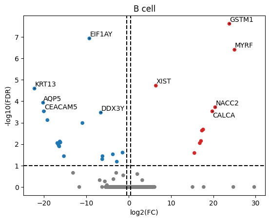
8. Make volcano plots#
Convert DE results to p-value/logFC matrices as used by decoupler
logFCs, pvals = aps.tl.long_form_df_to_decoupler(pd.concat(de_results.values()), p_col="padj")
Make a volcano plot for all cell-types of interest (e.g. B cells)
fig, ax = plt.subplots()
dc.plot_volcano(logFCs, pvals, "B cell", name="B cell", top=10, sign_thr=0.1, lFCs_thr=0.5, ax=ax)
ax.set_ylabel("-log10(FDR)")
ax.set_xlabel("log2(FC)")
fig.show()
Normalize pseudobulk to log counts per million (logCPM)
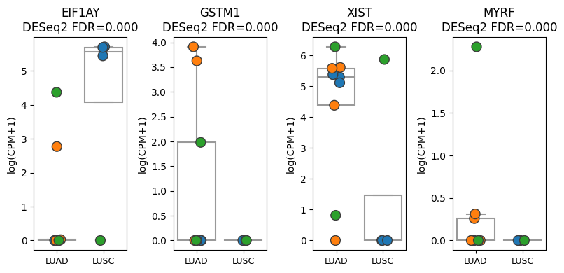
9. Plot genes of interest as paired dotplots#
Here, we are visualizing the actual expression values for each sample for all genes and cell-types of interest
Define list of genes to visualize
genes = ["EIF1AY", "GSTM1", "XIST", "MYRF"]
Normalize pseudobulk to counts per million (CPM)
for tmp_pdata in pdata_by_cell_type.values():
    sc.pp.normalize_total(tmp_pdata, target_sum=1e6)
    sc.pp.log1p(tmp_pdata)
Make plot (e.g. B cells)
# Get p-values for genes of interest
tmp_pvalues = de_results["B cell"].set_index("gene_id").loc[genes, "padj"].values

aps.pl.plot_paired(
    pdata_by_cell_type["B cell"],
    groupby="condition",
    var_names=genes,
    hue="dataset",
    ylabel="log(CPM+1)",
    panel_size=(2, 4),
    pvalues=tmp_pvalues,
    pvalue_template=lambda x: f"DESeq2 FDR={x:.3f}",
)